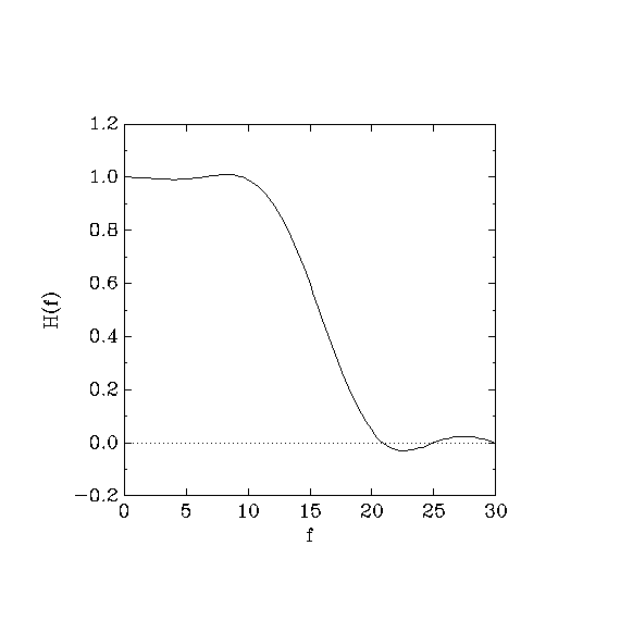
This example introduces point constraints. Even though a frequency response can only be approximated over a whole band, it is usually possible to specify an exact value of H(f) for a single frequency f, or for a finite set of frequencies. In this example, we design the same filter as in Example 2, but in addition, we specify that H(0) = 1 and H(25) = 0 exactly. These constraints are useful whenever we have noise at a known frequency (in our case, 25Hz) that we want to eliminate completely. The following specification file describes this design.
     (title "A simple filter III")
     (verbose #t)
     (cosine-symmetry)
     (filter-length 10)
     (sampling-frequency 60)
     (limit-= (band 0 10) 1 .2)
     (limit-= (band 20 30) 0)

     ;; We now constrain H(0) to be exactly 1.  We accomplish this effect
     ;; by setting weight = 0, and specifying the constraint for a point,
     ;; not for a band.
     (limit-= 0 1 0)

     ;; another point constraint at 25 Hz.  H(25) = 0.
     (limit-= 25 0 0)

     (output-file "example-3.coef")
     (plot-file "example-3.plot")
     (go)
A graph of the frequency response follows.

A point constraint is specified as in the command (limit-= 25 0
0). Note that we specify a single frequency 25 instead of a
band. gmeteor interprets this single frequency as the band
(band 25 25). Second, we set the weight to 0, so that the
constraint cannot be violated. (See Example 2, for a discussion
about weights.) With this change, we have |H(25)| = 0 exactly,
while in Example 2, we had |H(25)| = 0.008.