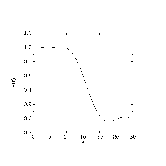
In this example, we introduce the concept of weight. Recall that in most cases, the desired frequency response can only be approximated. It turns out that the “optimal” approximation exhibits a ripple around the desired frequency response. Using weights, you can decrease the amplitude of the ripple within certain bands at the cost of a larger ripple amplitude in other bands. Specifically in this example, we want to reduce the approximation error in the passband at the expense of a larger error in the stopband, in such a way that the maximum error in the passband is one fifth of the maximum error in the stopband. This goal can be attained with the following specification file.
     ; parameters as in Example 1
     (title "A simple filter II")
     (verbose #t)
     (cosine-symmetry)
     (filter-length 10)
     (sampling-frequency 60)
     (output-file "example-2.coef")
     (plot-file "example-2.plot")

     ; new specifications
     (limit-= (band 0 10) 1 .2)   ; .2 is the weight
     (limit-= (band 20 30) 0)     ; no weight specified ==> weight = 1

     (go)
A graph of the frequency response follows.

Intuitively, this specification says that the passband [0..10] has
weight .2, and therefore the passband error will be one fifth of
the error in the stopband [20..30], where the weight is 1.
gmeteor always finds the filter that minimizes the error over the
whole frequency range. Unless you specify weights explicitly,
gmeteor distributes the error uniformly over all bands. If you
do specify weights, however, gmeteor spreads the error in each
band according to its weight.
The previous intuitive explanation suffices for simple cases, but we
need a more precise definition of a weight in order to design more
complicated filters. To this extent, we now discuss the operation of
gmeteor in more detail.
gmeteor's ultimate task is to find a frequency response
H(f) that satisfies certain upper- and lower-bound constraints.
For example, we might specify that H([0..10]) <= 1.1 and
that H([0..10]) >= 0.9. Whenever you specify equality
constraints with the limit-= command, gmeteor internally
converts them into a pair of inequality constraints. In our example,
gmeteor converts the specifications into the four constraints
H([0..10]) <= 1, H([0..10]) >= 1,
H([20..30]) <= 0, and H([20..30]) >=
0. Since these constraints are impossible to satisfy exactly with a
FIR filter, gmeteor somewhat relaxes these constraints in order
to compute the “optimal” approximation.
The constraint-relaxation algorithm works by introducing a
deviation parameter, denoted by y. Specifically in our
example, gmeteor rewrites the four constraints in this way:
H([0..10]) + w[1] y <= 1, H([0..10])
- w[2] y >= 1, H([20..30]) + w[3] y <=
0, and H([20..30]) - w[4] y >= 0. (Note that
the sign in front of w[i] y depends on the sense of the
inequality.) The parameters w[i] are the weights. In our
example, w[1] = w[2] = .2 and w[3] =
w[4] = 1.
The optimal filter is defined as the one that maximizes y.
The optimal y is negative whenever constraints are violated, as in our example. Since the absolute value of y denotes the maximum weighted distance between the desired and the actual frequency responses, maximizing y produces a filter with the minimum error, which is what we want. Designs where the optimal y is negative are instances of the approximation design style. (In Example 6, we show an example of a limit-style design where the constraints are not violated and y is positive. Even in that case, maximizing y turns out to be the right design criterion.)