2.6 Example 5

This example introduces concavity constraints. With gmeteor, you can impose constraints on the second derivative of the frequency response, in addition to constraints on the frequency response itself. These constraints are useful because a frequency response H that is either concave-up (i.e., H” >= 0) or concave-down (i.e., H” <= 0) in a certain band tends to be “flat” in that band (i.e., it does not exhibit ripples). (You can also impose constraints on the first derivative, but they do not appear to be very useful.)

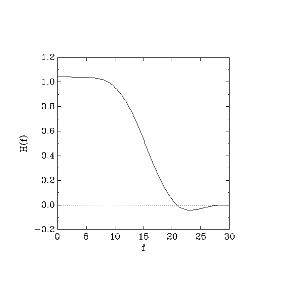
In this example, we design the low-pass filter from Example 1, but in addition we want a flat passband response. To accomplish this effect, we constrain the response to be concave-down in the passband.

     (title "A simple filter V")
     (verbose #t)
     (cosine-symmetry)
     (filter-length 10)
     (sampling-frequency 60)
     
     ;; magnitude constraints
     (limit-= (band 0 10) 1)
     (limit-= (band 20 30) 0)
     
     ;; This command states that H(f) must be concave down in the passband.
     ;; In other words, we demand that H''(f) <= 0 for f in the passband.
     (concave-down (band 0 10))
     
     (output-file "example-5.coef")
     (plot-file "example-5.plot")
     (go)

A graph of the frequency response follows.

The expression (concave-down band) specifies that the frequency response should be concave-down in the band band. The analogous command ‘concave-up’ does what you would expect. gmeteor also provides two commands ‘downward’ and ‘upward’ to impose constraints on H'(f).